Population Growth

Population ecologists make use of a variety of methods to model population dynamics mathematically. These more precise models can then be used to accurately describe changes occurring in a population and better predict future changes. Certain long-accepted models are now being modified or even abandoned due to their lack of predictive ability, and scholars strive to create effective new models.

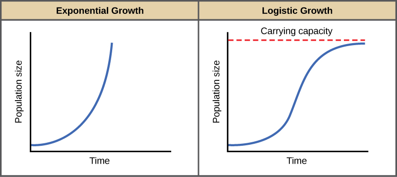
The simplest models of population growth use deterministic equations (equations that do not account for random events) to describe the rate of change in the size of a population over time. The first of these models, exponential growth, describes populations that increase in numbers without any limits to their growth. The second model, logistic growth, introduces limits to reproductive growth that become more intense as the population size increases. Neither model adequately describes natural populations, but they provide points of comparison.

Exponential Growth

Charles Darwin, in his theory of natural selection, was greatly influenced by the work of Thomas Malthus. Malthus published a book in 1798 stating that populations with unlimited natural resources grow very rapidly, which represents an exponential growth, and then population growth decreases as resources become depleted, indicating a logistic growth.

The best example of exponential growth is seen in bacteria. Bacteria reproduce by prokaryotic fission. This division takes about an hour for many bacterial species. If 1,000 bacteria are placed in a large flask with an unlimited supply of nutrients (so the nutrients will not become depleted), after an hour, there is one round of division and each organism divides, resulting in 2,000 organisms—an increase of 1,000. In another hour, each of the 2,000 organisms will double, producing 4,000, an increase of 2,000 organisms. After the third hour, there should be 8,000 bacteria in the flask, an increase of 4,000 organisms. The important concept of exponential growth is the accelerating population growth rate—the number of organisms added in each reproductive generation—that is, it is increasing at a greater and greater rate. After 1 day and 24 of these cycles, the population would have increased from 1,000 to more than 16 billion. When the population size, N, is plotted over time, a J-shaped growth curve is produced (Figure 13.1).

Reading Question #1

Why is the example about bacterial proliferation, given above, a good example of exponential growth? Select all that apply.

A. There is no limit in nutrient supply.
B. There is a strict limit in nutrient supply.
C. The rate at which the population grows increases over time.
D. The rate at which the population grows is constant over time.
E. The rate at which the population grows decreases over time.
F. Plotting the growth trend over time would result in an S-shaped curve.
G. Plotting the growth trend over time would result in an J-shaped curve.

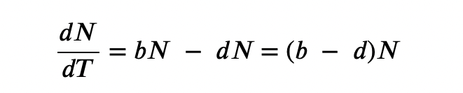
The bacteria example is a poor representation of the real world, in which resources are limited. Furthermore, some bacteria will die during the experiment and thus not reproduce, lowering the growth rate. Therefore, when calculating the growth rate of a population, the death rate (D) (number organisms that die during a particular time interval) is subtracted from the birth rate (B) (number organisms that are born during that interval). This is shown in the following formula:

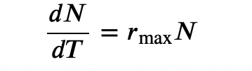
The birth rate is usually expressed on a per capita (for each individual) basis. Thus, B (birth rate) = bN (the per capita birth rate “b” multiplied by the number of individuals “N”) and D (death rate) = dN (the per capita death rate “d” multiplied by the number of individuals “N”). Additionally, ecologists are interested in the population at a particular point in time, an infinitely small time interval. For this reason, the terminology of differential calculus is used to obtain the “instantaneous” growth rate, replacing the change in number and time with an instant-specific measurement of number and time.

Notice that the “d” associated with the first term refers to the derivative (as the term is used in calculus) and is different from the death rate, also called “d.” The difference between birth and death rates is further simplified by substituting the term “r” (intrinsic rate of increase) for the relationship between birth and death rates:

The value of “r” can be positive, meaning the population is increasing in size; or negative, meaning the population is decreasing in size; or zero, where the population’s size is unchanging, a condition known as zero population growth. A further refinement of the formula recognizes that different species have inherent differences in their intrinsic rate of increase (often thought of as the potential for reproduction), even under ideal conditions. Obviously, a bacterium can reproduce more rapidly and have a higher intrinsic rate of growth than a human. The maximal growth rate for a species is its biotic potential, or r_max, thus changing the equation to:

Reading Question #2

What does the term r represent in exponential population growth equations? r represents the…

A. birth rate of the population
B. death rate of the population
C. number of individuals in the population
D. intrinsic rate of increase in the population

Logistic Growth

Exponential growth is possible only when infinite natural resources are available; this is not the case indefinitely in the real world. Charles Darwin recognized this fact in his description of the “struggle for existence,” which states that individuals will compete (with members of their own or other species) for limited resources. The successful ones will survive to pass on their own characteristics and traits (which we know now are transferred by genes) to the next generation at a greater rate (natural selection). To model the reality of limited resources, population ecologists developed the logistic growth model.

Carrying Capacity and the Logistic Model

In the real world, with its limited resources, exponential growth cannot continue indefinitely. Exponential growth may occur in environments where there are few individuals and plentiful resources, but when the number of individuals gets large enough, resources will be depleted, slowing the growth rate. Eventually, the growth rate will plateau or level off (Figure 13.1, right). This population size, which represents the maximum population size that a particular environment can support, is called the carrying capacity, or K.

The formula we use to calculate logistic growth adds the carrying capacity as a moderating force in the growth rate. The expression “K – N” indicates how many individuals could be added to a population at a given stage, and “K– N” divided by “K” is the fraction of the carrying capacity available for further growth. Thus, the exponential growth model is restricted by this factor to generate the logistic growth equation:

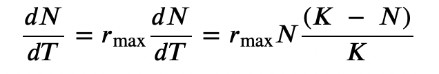
Notice that when N is very small, (K-N)/K becomes close to K/K or 1, and the right side of the equation reduces to r_maxN, which means the population is growing exponentially and is not influenced by carrying capacity. On the other hand, when N is large, (K-N)/K comes close to zero, which means that population growth will be slowed greatly or even stopped. Thus, population growth is greatly slowed in large populations by the carrying capacity, K. This model also allows for the population of a negative population growth, or a population decline. This occurs when the number of individuals in the population exceeds the carrying capacity (because the value of (K-N)/K is negative).

A graph of this equation yields an S-shaped curve (Figure 13.1, right), and it is a more realistic model of population growth than exponential growth. There are three different sections to an S-shaped curve. Initially, growth is exponential because there are few individuals and thus ample resources available. Then, as resources begin to become limited, the growth rate decreases. Finally, growth levels off at the carrying capacity of the environment, with little change in population size over time.

Role of Intraspecific Competition

The logistic model assumes that every individual within a population will have equal access to resources and, thus, an equal chance for survival. For plants, the amount of water, sunlight, nutrients, and the space to grow are the important resources, whereas in animals, important resources include food, water, shelter, nesting space, and mates.

In the real world, phenotypic variation among individuals within a population means that some individuals will be better adapted to their environment than others. The resulting competition between population members of the same species for resources is termed intraspecific competition (intra- = “within”; -specific = “species”). Intraspecific competition for resources may have little effect populations that are well below their carrying capacity—resources are plentiful and all individuals can obtain what they need. However, as population size increases, this competition intensifies. In addition, the accumulation of waste products can reduce an environment’s carrying capacity.

Examples of Logistic Growth

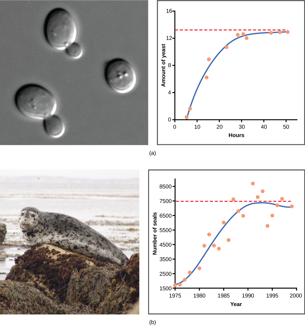
Yeast, a microscopic fungus used to make bread and alcoholic beverages, exhibits the classical S-shaped curve when grown in a test tube (Figure 13.2a). Its growth levels off as the population depletes the nutrients. In the real world, however, there are variations to this idealized curve. Examples in wild populations include sheep and harbor seals (Figure 13.2b). In both examples, the population size exceeds the carrying capacity for short periods of time and then falls below the carrying capacity afterwards. This fluctuation in population size continues to occur as the population oscillates around its carrying capacity.

Reading Question #3

In the logistic population growth equation, what does K represent? Select all correct answers.

A. Rate at which the population changes over time
B. Carrying capacity
C. Biotic potential
D. The greatest population of a species that can be maintained by a given environment
E. The maximum rate at which a species can grow in a given environment.

 

Population dynamics and regulation

The logistic model of population growth, while valid in many natural populations and a useful model, is a simplification of real-world population dynamics. Implicit in the model is that the carrying capacity of the environment does not change, which is not the case. Carrying capacity for naturally occurring populations can vary annually: for example, some summers are hot and dry whereas others are cold and wet. In many areas, the carrying capacity during the winter is much lower than it is during the summer. Also, natural events such as earthquakes, volcanoes, and fires can alter an environment and hence its carrying capacity. Additionally, populations do not usually exist in isolation. They engage in interspecific competition: that is, they share the environment with other species competing for the same resources. These factors are also important to understanding how a specific population will grow.

Population growth is regulated in a variety of ways. These are grouped into density-dependent factors, in which the density of the population at a given time affects growth rate and mortality, and density-independent factors, which influence mortality in a population regardless of population density. Note that in the former, the effect of the factor on the population depends on the density of the population at onset. Conservation biologists want to understand both types because this helps them manage populations and prevent extinction or overpopulation.

Density-dependent Regulation

Most density-dependent factors are biological in nature (biotic), and include predation, inter- and intraspecific competition, accumulation of waste, and diseases such as those caused by parasites. Usually, the denser a population is, the greater its mortality rate. For example, during intra- and interspecific competition, the reproductive rates of the individuals will usually be lower, reducing their population’s rate of growth. In addition, low prey density increases the mortality of its predator because it has more difficulty locating its food source.

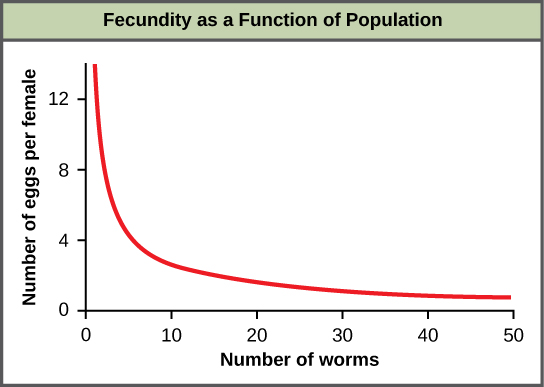
An example of density-dependent regulation is shown in Figure 13.3 with results from a study focusing on the giant intestinal roundworm (Ascaris lumbricoides), a parasite of humans and other mammals. Denser populations of the parasite exhibited lower fecundity; they contained fewer eggs. One possible explanation for this is that females would be smaller in more dense populations (due to limited resources) and that smaller females would have fewer eggs. This hypothesis was tested and disproved in a 2009 study which showed that female weight had no influence. The actual cause of the density-dependence of fecundity in this organism is still unclear and awaiting further investigation.

Density-Independent Regulation and Interaction with Density-Dependent Factors

Many factors, typically abiotic (e.g., physical or chemical), influence the mortality of a population regardless of its density, including weather, natural disasters, and pollution. An individual deer may be killed in a forest fire regardless of how many deer happen to be in that area. Its chances of survival are the same whether the population density is high or low. The same holds true for cold winter weather.

In real-life situations, population regulation is very complicated and density-dependent and independent factors can interact. A dense population that is reduced in a density-independent manner by some environmental factor(s) will be able to recover differently than a sparse population. For example, a population of deer affected by a harsh winter will recover faster if there are more deer remaining to reproduce.

Connection to Evolution

Why Did the Woolly Mammoth Go Extinct?

 

 

It’s easy to get lost in the discussion about why dinosaurs went extinct 65 million years ago. Was it due to a meteor slamming into Earth near the coast of modern-day Mexico, or was it from some long-term weather cycle that is not yet understood? One hypothesis that will never be proposed is that humans had something to do with it. Mammals were small, insignificant creatures of the forest 65 million years ago, and no humans existed. Scientists are continually exploring these and other theories.

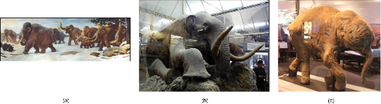
Woolly mammoths began to go extinct much more recently, about 10,000 years ago, when they shared the Earth with humans who were no different anatomically than humans today (Figure 13.4). Mammoths survived in isolated island populations as recently as 1700 BC. We know a lot about these animals from carcasses found frozen in the ice of Siberia and other regions of the north. Scientists have sequenced at least 50 percent of its genome and believe mammoths are between 98 and 99% identical to modern elephants.

It is commonly thought that climate change and human hunting led to their extinction. A 2008 study estimated that climate change reduced the mammoth’s range from 3,000,000 square miles 42,000 years ago to 310,000 square miles 6,000 years ago  (Nogués-Bravo et al. 2008). It is also well documented that humans hunted these animals. A 2012 study showed that no single factor was exclusively responsible for the extinction of these magnificent creatures. In addition to human hunting, climate change, and reduction of habitat, these scientists demonstrated another important factor in the mammoth’s extinction was the migration of humans across the Bering Strait to North America during the last ice age 20,000 years ago.

The maintenance of stable populations was and is very complex, with many interacting factors determining the outcome. It is important to remember that humans are also part of nature. We once contributed to a species’ decline using only primitive hunting technology.

References

Adapted from

Clark, M.A., Douglas, M., and Choi, J. (2018). Biology 2e. OpenStax. Retrieved from https://openstax.org/books/biology-2e/pages/45-3-environmental-limits-to-population-growth

and

Fisher, M.R., and Editor. (n.d.) Environmental Biology. PressBooks. Retrieved from https://iu.pressbooks.pub/environmentalbiology/chapter/4-2-population-growth-and-regulation/